Don’t Widen the Road

This post is part one of a two-part post (part two) on why I am not looking forward to the future of autonomous cars. That opinion in itself is far from uncommon, but everyone else I’ve met who feels the same way has justified it with one or more of these three reasons:

1. They don’t trust its safety
2. They will miss driving
3. They are afraid of the job obsolescence that will come with it

While I do belong to the last of those groups, that’s not my main concern. It often catches people off guard when I say something along the lines of “I think autonomous cars will be safer and cause less congestion per vehicle than human drivers, but I still think they’ll make things worse.” Here, I’m aiming to justify that opinion. This first piece will focus on a point that will act as a foundation for the next post. I kept them separate because I think both make valuable points on their own.

The focus of this post is why widening roads is a counterproductive practice. In the USA, the prevailing assumption seems to be more lanes = faster commute (growing up in a town where the interstate highway notoriously drops from three to two lanes probably magnified this as well). This is hardly a surprise in what is by far the most car-centric country in the world, but it did make for a bit of a shock when I learned more about the subject and realized that assumption is wrong. 

The short justification for why widening roads doesn’t help is the economic idea of induced demand (a search for this will give plenty of sources on this subject), which is basically to say: if travel along a road becomes faster, more people will take that route, making traffic increase again. While this is the gist of the matter, this really only explains the “what”, and not the “how”, so here I will give a more comprehensive explanation of this idea.

When studying and quantifying physical systems, a common idea that arises is steady state vs. transient state. Steady state is the state of the system once it’s no longer changing, while transient state is the state of it while it’s still changing. For example, take an ice cube placed in a room-temperature chamber where heat can’t escape (idealized). Here, you could come up with a set of transient equations that describe the temperature of the ice cube and the air over time while the ice cube melts, and you could also find the steady state of the system, which would simply be the temperature of the air and water once they reached the same temperature and heat was no longer passing between them.  Assuming no heat transfer into/out of the chamber, as we did, the steady state would persist indefinitely. At steady state, a system is said to be in equilibrium.

Socioeconomic systems similarly have transient and steady states, and the basis of my explanation here is that widening roads can result in shorter commute times in the transient state, but is useless once equilibrium is reached. Transient state, by definition, is not sustainable, and real solutions need to focus on the impact had on the equilibrium. I have a suspicion that humans’ difficulty in recognizing transient vs. steady state impacts is one of our biggest barriers to creating a better future. This post focusses on one example, but it’s not difficult to apply the concept to such topics as economic and environmental policy.

To start describing the particular socioeconomic system at play here, let’s first look at how people decide where to live. For most people, the decision comes down to some combination of the following factors:

• Price of the place (rent/mortgage + taxes + utilities)
• Resulting commute to work and other commonly visited places (monetary cost + time cost)
• Cost of maintaining the place (monetary + time as well)
• Quality of the neighborhood (based on preferences, e.g. quiet, safe, near downtown, etc.)
• Quality of the specific apartment/house

Given these factors, you could theoretically come up with an equation for the total cost of a place by quantifying each of these factors and weighting them. Let’s call this the PCC equation, for Personal Cumulative Cost. Each person would have their own PCC equation, and the cheaper the PCC of a place, the more desirable it would be to live at. People who are looking to move will move to the place with the cheapest PCC that they can find, and people who aren’t actively looking to move will still move if there’s a large enough differential in PCC between their current place and another place.

You may have already gathered that for many people, the PCC of a place depends on the typical traffic between it and their workplace, gym, grocery store, relatives & friends, beach, etc., which is how this all ties together. When a highway gets a new lane, commute times will reduce along that highway (transiently), which means dwellings that would require use of that highway would drop in PCC.

Before going further, I should concede that in the real world a true equilibrium of this system of where people live & how they commute is basically unachievable, because much more than just road widths determine it. However, one of the most elementary concepts in science is isolating variables, so in this thought experiment I am assuming nothing is changing in this system other than road widths.

Getting back on track, let’s create a specific example to assist in describing the system. We’ll have two towns, A and B, connected by a single highway, 1. I’m sure you’re able to picture this on your own, but I like schematics, so here’s one for this example:

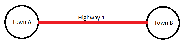
Let’s assume A and B are roughly equivalent in terms of location relative to amenities, safety, quality & size of houses/apartments, and size. However, B has far more jobs than A. I haven’t said anything about housing prices yet, but if we first ignore that, B would clearly have more people wanting to live there, as the “commute” portion of the PCC equation would favor B for most people, and everything else (again, other than price) is equal between the two. However, as I said, the towns are equal size, so some people must live in A and work in B. These people, if presented with equivalent places in either town for equal price, would choose the one in B, so one of the following two forces must be at play to have them end up in A:

1. There weren’t any places available in B
2. The place in A was cheaper than the place in B

Unless local laws or geography prevent it, force 1 will usually resolve itself via new housing developments in B to meet the demand. Further, if this wasn’t resolved via increasing supply, prices would naturally increase there anyway, so ultimately force 2 is what would happen. So there we have it – people are split between A and B based on how their PCC equation weights different factors, with the basic tradeoff being that A is cheaper to live in than B, with the caveat that you have a longer commute on the congested Hwy 1.

We come to equilibrium when this equilibrium condition is met: Everyone whose PCC is cheaper in A lives in A and everyone whose PCC is cheaper in B lives in B. Then one day, the state allocates $500 million to widen Hwy 1 “to reduce commute times” between A and B. Residents of A applaud it, as a shorter commute time means the PCC of their house is now much less than one in B that was previously roughly equivalent. Great!

This only lasts until the residents of B realize there’s places in A cheaper, in terms of PCC, than their place and start to move the A because of it. This is the transient state of A & B, which lasts until the equilibrium stated above is once again met. The key point to keep in mind here is that the PCC equations have not changed through all this, only the inputs (the factors listed) change. This means people will move until those inputs once again reach a steady state, which we are not in when we introduce a disturbance like a commute time change.

So what can change to return us to steady state? Well, the neighborhoods and houses themselves are not changing, so the only factors that can really change are housing prices and commute times. In other words, people are going to move from B to A until A gets so expensive it’s not worth moving there, or the commutes get bad enough it’s not worth moving there, or a combination of the two.

If prices in A stay the same, then the commute time at which no one from B will want to move to A is exactly the commute time we had to start, when no one from B wanted to move to A. So that means if prices don’t rise in A, people will move there until Hwy 1 is just as congested as before. In this way, the congestion level of Hwy 1 is more of a function of the housing/job market and the priorities of the residents of its surrounding population centers than it is of its number or lanes.

Of course, I made a huge assumption by saying the prices in A would stay the same, so let’s consider the alternative. If A becomes more expensive, the commute time will need to be faster than the initial (pre-widening) commute time was, or no one would move there from B. This could be seen as a point of hope, but it shouldn’t be. What this is effectively doing is pricing people out of using Hwy 1 – people who would’ve moved to A if it was a little cheaper won’t because it’s not worth it at its new housing price. If we’re content with pricing people out of Hwy 1 as a way to reduce its traffic, there’s another solution that’s better in every way I can think of: make Hwy 1 a toll road. This way you’re bringing in money, hopefully to be spent for the public good, rather than expending money on a useless project that destroys natural habitats and leads to more pollution because of more people driving. 

At this point, you may be wondering what can be done to improve traffic, aside from making toll roads as stated. To get to that, I should first summarize the main point of this post as follows: the amount of traffic will settle itself at the worst point where people still choose driving over alternatives. This presupposes there’s enough supply of drivers to cause traffic, which is true for any metropolitan area, but likely not true for rural towns, but rural towns are never the ones widening roads anyway. The main implication here is that traffic is a function of human priority setting, not how roads are built. So, the only way to reduce traffic is to make driving less desirable. You can do that by making alternatives more desirable (increasing public transportation, adding bike lanes + pedestrian paths) or by directly making driving less desirable (higher gas taxes, toll roads).  Maybe if we banned speakers, AC & heaters in cars it would solve our traffic problems!

In my next post, I’ll use the PCC idea to explain the likely outcomes of the rise of autonomous cars.